Tuesday, October 25, 2022

Auto Format Row & Coloumn Colour with Mouse Click In Excel

Tutorial on auto format of complete row and column colour of cell which we click.


We have explain the each step in very easiest way including how to activate developer tab in microsoft excel, we have also added VBA code below which can be just copied and pasted.


Copy the code from below and paste it under sheet which hold data:


Private Sub Worksheet_SelectionChange(ByVal Target As Range)

If Application.CutCopyMode = False Then

Application.Calculate

End If

End Sub


Formula for Coloumn: =COLUMN()=CELL("col") Formula for Row: =CELL("row")=ROW()


To download sample file ➡ Click Here  (Download the file and open in excel to make it work)


Sunday, October 23, 2022

MS EXCEL - SPEEDOMETER CHART TUTORIAL

SPEEDMETER CHART FOR DYNAMIC INTERACTIVE DASHBOARD IN EXCEL


Blog coming soon, mean while checkout our new tutorial under below video and to download sample file: ➡ Click Here 

Note: Download the file and open in EXCEL to use the chart


Wednesday, October 19, 2022

Tutorial - Link Checkboxes To Multiple Cells In Excel

 Tutorial - How To Link Checkboxes To Multiple Cells In Excel


*To Add Checkboxs Under Multiple Range Click Here*


If there are thousands checkboxes need to be linked to other cells, you can apply the following VBA code, and to apply code follow the below step.


1. Go to your worksheet and create checkboxes.

2. Hold down the ALT + F11 keys to open the Microsoft Visual Basic for Applications window or you can click on Developer tab ➡ Visual Basic.


3. Click Insert > Module


4. Double click on module1 and paste the below code in the Module Window (make sure module window is clear)
Sub LinkChecks()
'Update by Extendoffice
Dim xCB
Dim xCChar
i = 2
xCChar = "B"
For Each xCB In ActiveSheet.CheckBoxes
If xCB.Value = 1 Then
    Cells(i, xCChar).Value = True
Else
    Cells(i, xCChar).Value = False
End If
xCB.LinkedCell = Cells(i, xCChar).Address
i = i + 1
Next xCB
End Sub

4. And then press F5 key to run this code,now all the checkboxes in the active worksheet have been linked to the cells, when you check the checkbox, its relative cell will display TRUE, if you clear a check box, the linked cell should show FALSE.


Note: In the above code, i = 2, the number 2 is the starting row of your checkbox, and the letter B is the column location where you need link the checkboxes to. You can change them to your need.


To Learn How To Add Multiple Checkbox Check Below Video:


Monday, October 17, 2022

Ms Excel- Dynamic Dashboard - Tutorial 01

 How to create speedometer in ms excel - Tutorial


Before we move on to Dynamic Dashboard will learn how to create speedometer chart.

To add the chart on our excel we need below data on our sheet!


Speedometer category:    
Bad
Average
Good
Excellent


Names             Range 
Needle               45%
Needle Size         1%
Blank Area        154%


Now create a SPEEDOMETER in Excel,use the below steps:

1. Go to Insert Tab ➡ Charts ➡ Doughnut Chart (you will get a blank chart area)


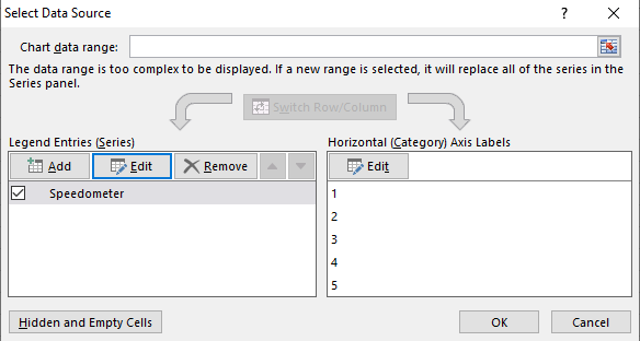
2. Right click on the blank chart and then click on Select Data.

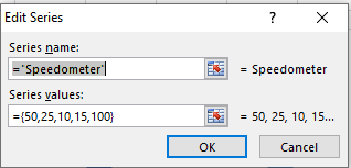
3. New window will popup and under that window click Add button and then under series name type any name " we added speedometer", under series range type ={50,25,10,15,100} and hit ok as shown in image below:

Once you done you popup box should look like below and then hit okay.

Once you click okay, your doughnut chart will like below (After deleting label)

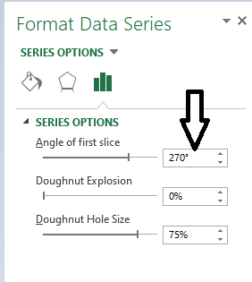
4. Now change the angle of the chart and for that right click on the chart and then click on Format Data Series ➡ type 270° under “Angle of first slice”  and change the Doughnut hole size to 60% then hit enter

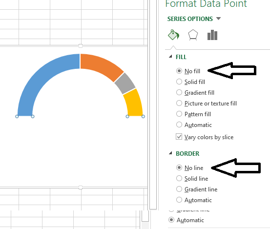
5. Click on the below part of chart which is not required and click on fill option click "No Fill", do the same for border.


6. Repeat the same for rest of the area and select solid colour and use the same for border we have used the colour as below you can any of your choice:
7. Now it's time to create needle for you meter and do add that will add pie chart on same chart area by right click on chart and click select data.
Under popup window click on "Add button" ➡ Under series name type "Needle" and under range select the range from Sheet then hit okay.

Your chart should look like this:
8. Now it's time to merge the charts, to do so ➡ 
Design Tabs ➡ Change Chart Type. Under new pop window click combo ➡ select  Doughnut for Speedometer and Pie for Needle then hit okay

9. Now again select the pie chart right click on it ➡ format data series and unfill the major part of chart and keep the smallest part by filling it color as black. 
Note: If after selecting a pie chart if the angle is not correct  make sure to change it to 270* for both the charts.

10. At this movment your chart should look like below:
11. Now it's time to add label and to do that 
Right Click ➜ Add Data Labels ➜ Add Data Labels ➡ select the data labels ➡ Format Data Label and after that click on Values from Cells then label from the first sheet and untick Values.

Once It's done your speedometer is ready you can watch our tutorial video for details - Click Here ▶


Sunday, October 9, 2022

Tutorial - How To Convert Number To Words In Excel

Watch out video, how to apply below code.


Copy the below code and paste under module 


Public Function Spellnumber(SNum As String)

'Updateby Extendoffice

Dim xDPInt As Integer

Dim xArrPlace As Variant

Dim xRStr_  As String

Dim xNumStr As String

Dim xF As Integer

Dim xTemp As String

Dim xStrTemp As String

Dim xRStr As String

Dim xLp As Integer

xArrPlace = Array("", "", " Thousand ", " Lacs ", " Crores ", " Trillion ", "", "", "", "")

On Error Resume Next

If SNum = "" Then

  Spellnumber = ""

  Exit Function

End If

xNumStr = Trim(Str(SNum))

If xNumStr = "" Then

  Spellnumber = ""

  Exit Function

End If


xRStr = ""

xLp = 0

If (xNumStr > 999999999.99) Then

    Spellnumber = "Digit excced Maximum limit"

    Exit Function

End If

xDPInt = InStr(xNumStr, ".")

If xDPInt > 0 Then

    If (Len(xNumStr) - xDPInt) = 1 Then

       xRStr_ = Spellnumber_GetT(Left(Mid(xNumStr, xDPInt + 1) & "0", 2))

    ElseIf (Len(xNumStr) - xDPInt) > 1 Then

       xRStr_ = Spellnumber_GetT(Left(Mid(xNumStr, xDPInt + 1), 2))

    End If

        xNumStr = Trim(Left(xNumStr, xDPInt - 1))

    End If

    xF = 1

    Do While xNumStr <> ""

        If (xF >= 2) Then

            xTemp = Right(xNumStr, 2)

        Else

            If (Len(xNumStr) = 2) Then

                xTemp = Right(xNumStr, 2)

            ElseIf (Len(xNumStr) = 1) Then

                xTemp = Right(xNumStr, 1)

            Else

                xTemp = Right(xNumStr, 3)

            End If

        End If

        xStrTemp = ""

        If Val(xTemp) > 99 Then

            xStrTemp = Spellnumber_GetH(Right(xTemp, 3), xLp)

            If Right(Trim(xStrTemp), 3) <> "Lac" Then

            xLp = xLp + 1

            End If

        ElseIf Val(xTemp) <= 99 And Val(xTemp) > 9 Then

            xStrTemp = Spellnumber_GetT(Right(xTemp, 2))

        ElseIf Val(xTemp) < 10 Then

            xStrTemp = Spellnumber_GetD(Right(xTemp, 2))

        End If

        If xStrTemp <> "" Then

            xRStr = xStrTemp & xArrPlace(xF) & xRStr

        End If

        If xF = 2 Then

            If Len(xNumStr) = 1 Then

                xNumStr = ""

            Else

                xNumStr = Left(xNumStr, Len(xNumStr) - 2)

            End If

       ElseIf xF = 3 Then

            If Len(xNumStr) >= 3 Then

                 xNumStr = Left(xNumStr, Len(xNumStr) - 2)

            Else

                xNumStr = ""

            End If

        ElseIf xF = 4 Then

          xNumStr = ""

    Else

        If Len(xNumStr) <= 2 Then

        xNumStr = ""

    Else

        xNumStr = Left(xNumStr, Len(xNumStr) - 3)

        End If

    End If

        xF = xF + 1

Loop

    If xRStr = "" Then

       xRStr = "No"

    Else

       xRStr = xRStr

    End If

    If xRStr_ <> "" Then

       xRStr_ = " Point " & xRStr_ & "  "

    End If

    Spellnumber = xRStr & xRStr_

    End Function

Function Spellnumber_GetH(xStrH As String, xLp As Integer)

Dim xRStr As String

If Val(xStrH) < 1 Then

    Spellnumber_GetH = ""

    Exit Function

Else

   xStrH = Right("000" & xStrH, 3)

   If Mid(xStrH, 1, 1) <> "0" Then

        If (xLp > 0) Then

         xRStr = Spellnumber_GetD(Mid(xStrH, 1, 1)) & " Lac "

        Else

         xRStr = Spellnumber_GetD(Mid(xStrH, 1, 1)) & " Hundred "

        End If

    End If

    If Mid(xStrH, 2, 1) <> "0" Then

        xRStr = xRStr & Spellnumber_GetT(Mid(xStrH, 2))

    Else

        xRStr = xRStr & Spellnumber_GetD(Mid(xStrH, 3))

    End If

End If

    Spellnumber_GetH = xRStr

End Function

Function Spellnumber_GetT(xTStr As String)

    Dim xTArr1 As Variant

    Dim xTArr2 As Variant

    Dim xRStr As String

    xTArr1 = Array("Ten", "Eleven", "Twelve", "Thirteen", "Fourteen", "Fifteen", "Sixteen", "Seventeen", "Eighteen", "Nineteen")

    xTArr2 = Array("", "Twenty", "Thirty", "Forty", "Fifty", "Sixty", "Seventy", "Eighty", "Ninety")

    Result = ""

    If Val(Left(xTStr, 1)) = 1 Then

        xRStr = xTArr1(Val(Mid(xTStr, 2, 1)))

    Else

        If Val(Left(xTStr, 1)) > 0 Then

            xRStr = xTArr2(Val(Left(xTStr, 1)) - 1)

        End If

        xRStr = xRStr & Spellnumber_GetD(Right(xTStr, 1))

    End If

      Spellnumber_GetT = xRStr

End Function

Function Spellnumber_GetD(xDStr As String)

Dim xArr_1() As Variant

    xArr_1 = Array(" One", " Two", " Three", " Four", " Five", " Six", " Seven", " Eight", " Nine", "")

    If Val(xDStr) > 0 Then

        Spellnumber_GetD = xArr_1(Val(xDStr) - 1)

    Else

        Spellnumber_GetD = ""

    End If

End Function


How To Use Vlookup In Merged Cells

  How To Use Vlookup In Merged Cells Click Here to download sample file for practice Note: Download the file and open with microsoft excel